
At Hot Chips 2026, Agentrys presented an autonomous chip optimization workflow built on Agentrys Studio. We applied it to XiangShan, a Linux-class RISC-V processor, with the goal of improving performance, power, and area for a specific workload. The workflow autonomously proposed and evaluated design changes using correctness checks, synthesis, place-and-route, and timing analysis. In eight hours, it found a configuration that improved throughput by 40% while reducing power by 28% and area by 10% relative to the reference design.
expert-tuned reference
at the same time
reference stops at 1.22
tuning loop
This work demonstrates loop engineering: designing the objectives, actions, evaluators, state, and failure-handling mechanisms that connect each result to the next design change.
Chip design is a strong environment for loop engineering because proposed changes can be executed and measured. Compilers and simulators check function; synthesis and physical design measure timing, power, and area. The difficulty is integrating these tools into a reliable feedback loop when evaluations are expensive, failures are common, and many proposed designs are invalid.
Another example from Hot Chips 2026 was OpenAI’s Jalapeño, an inference ASIC built with AI in the design loop. As reported from the session by ServeTheHome and Tom’s Hardware,1 OpenAI stated measured block-level wins over a human baseline — 56% on a BF16 multiply, alongside a 10% smaller matrix-unit area — within a roughly nine-month path from RTL to tapeout.
The design and the workload
The target was OpenXiangShan XiangShan (kunminghu-v3, fixed commit): an RV64GC out-of-order core with approximately 143k lines of Chisel in 528 source files. The workflow extracted 3,284 parameters and grouped them into 17 microarchitectural subsystems.
The primary workload was GAP BFS: Graph500-style RMAT breadth-first search at scale 14 (16,384 vertices; 262,144 edges). It is memory-latency-bound and stresses the reorder buffer, load/store queues, memory-level parallelism and cache hierarchy. LLM token decode and a branch-heavy workload provided secondary coverage.
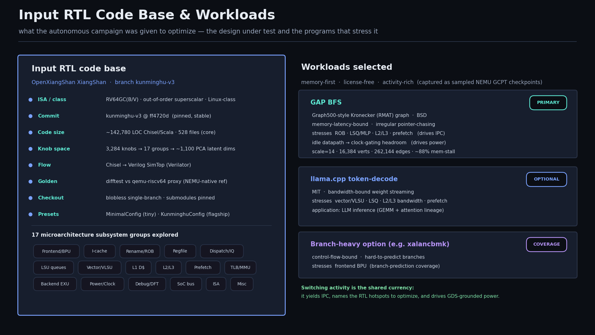
GAP BFS spent approximately 88% of cycles stalled on memory. Structures outside the stall path therefore added power and area with limited performance benefit.
What we achieved
The workflow jointly optimizes microarchitectural parameters and RTL transforms against workload-dependent throughput, power, frequency and area. Each reported candidate passes correctness, synthesis, place-and-route and physical analysis on the same flow.
Comparison with the reference configuration
Both designs use the same RV64GC core, GAP BFS workload, standard-cell library and measurement flow. The reference reaches 1.22 GHz; the selected configuration closes at 1.53 GHz with higher IPC, lower power and lower area.
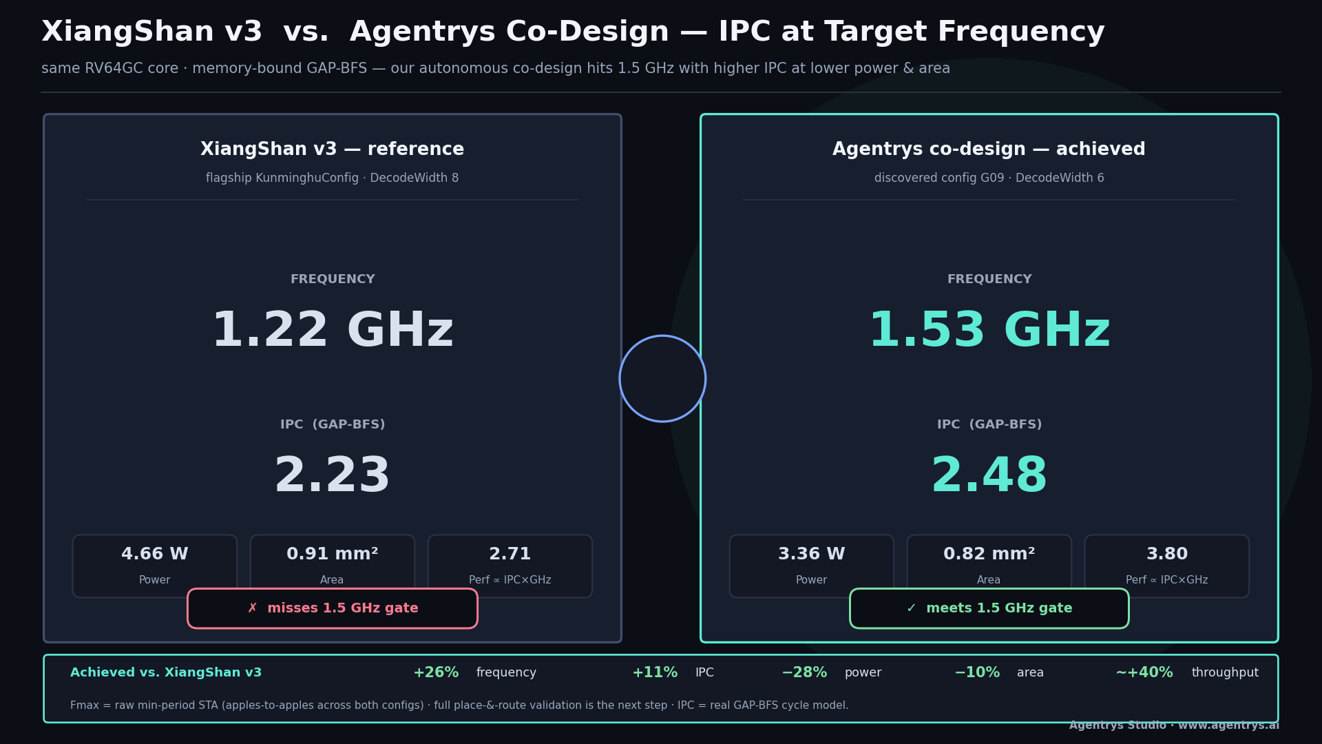
The gain comes from interacting parameter changes rather than a single adjustment, which makes one-parameter sweeps inadequate.
A trade-off frontier, not one configuration
The run retained all non-dominated configurations. Each point passed the same correctness and physical-analysis flow.
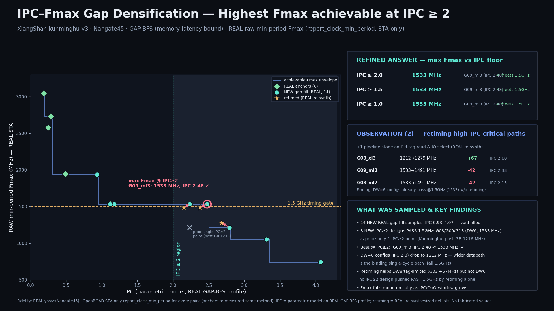
Wide, high-IPC configurations failed the 1.5 GHz constraint. Several narrower configurations closed above 1.5 GHz with IPC ≥ 2.
The minimum-energy point measured 0.84 W and 0.134 mm² while closing at 1.5 GHz, but at lower throughput than Figure 2. Energy-to-solution is derived from measured power and execution time, allowing the same frontier to be ranked by power, energy or throughput.
| Deliverable | What it contains |
|---|---|
| Trade-off frontier | The non-dominated set of buildable designs over all four objectives |
| Per-design artifacts | Layout, netlist, and power / timing / area reports for every frontier point |
| Discovered transforms | The hardware rewrites the loop found, with measured savings |
| Reproducibility manifest | Pinned inputs and full provenance to rebuild any point |
How the loop works
Microarchitecture design hides two optimization problems inside each other. The first is a choice of parameters: cache geometries, queue depths, register-file sizes, fetch, issue and decode widths. The second is the quality of the RTL that implements any given choice. The two are not separable, because the best size for a structure depends on how efficiently that structure is written, and how it is written changes what size is worth choosing. The workflow therefore optimizes both together, with one loop nested inside the other.
The outer loop searches the parameter space. The inner loop edits the RTL of the configuration the outer loop is currently examining. A single evaluator scores both: it takes a design through compilation, cycle-accurate simulation, synthesis, and place-and-route, then reads power, timing and area off the routed netlist. That physical result is what a candidate is judged on; no analytical proxy stands in for it at the moment of scoring.
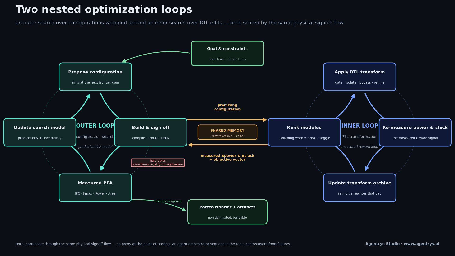
Outer loop: configuration search
Every tunable value the RTL exposes is a knob — a cache’s associativity, a queue’s depth, the number of physical registers, the decode and issue widths, a predictor table’s size. Read straight out of the Chisel source, they number 3,284. A configuration is one joint setting of all of them: a single group of microarchitectural knobs that together specify one buildable core. The outer loop searches the space of those configurations.
That space resists the usual tools. The knobs are discrete and mutually constrained — a queue depth has to divide an issue width, a cache geometry has to satisfy the coherence protocol — so there is no smooth surface for a numeric optimizer to descend, and much of the volume is not even legal to build. Brute force is no better: because scoring one configuration means a full synthesis-and-route, an exhaustive or densely random sweep over 3,284 dimensions would cost orders of magnitude more compute than the problem can justify. Neither continuous approximation nor blanket enumeration is viable.
The way through is to shrink the space without throwing away what matters. The 3,284 knobs are partitioned into 17 microarchitectural subsystems — front end, caches, instruction window, register file, load/store queues, and the rest — and within each subsystem the correlated knobs are projected onto a compact latent basis that preserves roughly 95% of their variation. This collapses 3,284 raw dimensions to about 1,100 searchable coordinates, each still traceable back to the named knobs it summarizes. An intractable space becomes one an optimizer can actually cover.
Search then runs in rounds. Each round builds a small batch of configurations — four, here — through the full flow and reads back the four objectives (IPC, frequency, power, area). Between rounds, an intelligent selector decides what to build next. It is a Bayesian-optimization model: from the results gathered so far it predicts, for any point in the latent space, each objective and how uncertain that prediction is. Its incentive is explicit — it proposes the configurations expected to expand the Pareto frontier the most, a criterion that simultaneously rewards designs predicted to be strong (exploitation) and designs where the outcome is most uncertain and therefore most informative (exploration). Only feasible, gate-passing results are fed back, so the model learns the shape of the buildable region rather than a fantasy of it. The outer loop is, in sum, a batch of real builds with an intelligent model choosing the next batch in between.
The payoff is sample efficiency: roughly fifty real builds were enough to reach the frontier shown earlier, where a grid at comparable resolution would have needed orders of magnitude more. What the loop cannot do is set by what the RTL exposes — it can resize the register file but not make the register file cheaper to write, and it cannot shorten a priority encoder on the critical path. Improving the implementation itself is the inner loop’s job.
Inner loop: RTL transformation
For a given configuration, the inner loop reads per-module switching activity from simulation and ranks modules by switching work — cell area weighted by toggle rate — which locates where dynamic energy is actually dissipated rather than where a designer expects it. The modules at the top of that ranking are its high-switching modules, and they are what the loop edits. The transforms are individually familiar: clock gating for logic that toggles while idle, operand isolation ahead of datapaths whose result is discarded, dataflow bypass, register forwarding, retiming, and removal of logic that cannot affect an output. The toolbox is standard; what the loop has to decide is which transform to apply to which high-switching module. Rather than follow a fixed rulebook, it tries candidate transforms on each one and keeps whichever yields the largest measured saving. Every edit is scored by pushing the resulting toggle profile back through the same activity-to-power calculation used at signoff, so a reported saving is a re-derived power number, not a heuristic credit.
Successful transforms are stored in an archive indexed by type and by the reduction they achieve; the best operator in each cell is reapplied when a similar high-switching module recurs on a later configuration, which spares the loop from rediscovering it. Retiming is the exception that proves useful for a different reason: it trades pipeline depth for a shorter critical path, improving frequency rather than power, and can move a configuration that narrowly failed timing across the target.
Shared memory between the loops
Run back to back, the two loops would each start cold and repeat the other’s work. Instead a persistent shared memory links them — not RAM, but a store of what has been learned so far, which both loops read and write for the whole run. It holds two things: an archive of the RTL rewrites proven to work on a given kind of high-switching module, and the inner loop’s measured results. When a similar module recurs on a later configuration, its proven transform is pulled from the archive instead of being rediscovered; and the power and slack the inner loop recovers are written back into the objective vector the outer model is fit on, so the outer search sees each configuration as it will actually be implemented, not as first drafted.
This buys the two things an expensive search most needs. Reusing solved sub-problems lets it converge faster — the same work is never paid for twice, which is precisely the idea of memoization in dynamic programming: overlapping sub-problems whose solutions are cached and reused. Folding the inner loop’s gains into the outer model makes it more accurate — the model learns the landscape of improved designs rather than of the raw RTL, so each proposal targets the frontier that is genuinely reachable. The reuse here is heuristic rather than a provable recurrence, so it is memoization in spirit rather than textbook dynamic programming — but the payoff is the same, and it shows up in the result: the frontier contains designs that no setting of the exposed parameters could reach alone, because part of each design’s quality came from RTL the inner loop rewrote and the shared memory carried forward.
Feasibility and its gates
Correctness and buildability are preconditions, not objectives, and are enforced as an ordered filter that a candidate clears before it is scored. The evaluation chain is arranged so the inexpensive checks reject first:
- Correctness — reproduce the golden reference model’s results.
- Legality — elaborate into a synthesizable design.
- Timing — close at the target frequency in post-route analysis.
- Liveness — complete the flow within its resource budget.
A configuration that fails elaboration never reaches the router, and the outer model is fit only on candidates that passed all four checks. Timing was the gate that repeatedly mattered: several configurations with high predicted IPC failed post-route closure, and a reward scored on a pre-layout estimate would have promoted them into the frontier. Requiring real closure is what kept them out.
Execution
Because physical evaluation dominates wall-clock time, configurations are built in parallel batches with the cheap gates ahead of emulation and routing. Specialized agents and deterministic scripts perform compilation, simulation, activity extraction, synthesis, routing and report parsing; an orchestrator dispatches them, validates each output, and retries, diagnoses or discards on tool failure. The single design objective of this layer is to spend a fixed compute budget on the evaluations most likely to extend the frontier.
In the work described here the workflow was fixed: the two loops optimized within an architecture specified in advance. A longer-term direction is to optimize the workflow itself — exploring alternative arrangements of agents and loops and evaluating which ones work better. The results in this article come from the two loops above, not from that outer layer.
Convergence
The stopping criterion is the change in dominated objective-space volume. The run ends when improvement remains below a threshold; this run converged before exhausting its evaluation budget.
Frontier convergence
Illustrative normalized dominated volume versus generation; not measured convergence data from this run.
A 1.5 GHz constraint removes the wide-machine region; a power constraint selects points closer to the minimum-energy end. Each frontier point is legal, correctness-verified and timing-closing, with artifacts and provenance.
Workflow portability
The workflow interfaces separate orchestration from the design, workload, implementation target and toolchain. Components can include open-source or proprietary tools, internal scripts, reference models and external agents. This experiment used an open-source ASIC flow; the same interface model supports other toolchains and FPGA targets.
A new design, workload or constraint set requires a new run and produces a different frontier.
Platform implementation
The Agentrys Studio Platform coordinated agents, tools, artifacts and evaluation results. Architects supplied the workload, objectives, constraints and implementation methodology; the workflow executed the design iterations and produced the frontier for review.
The broader lesson is that capable AI models are only one part of autonomous engineering. Useful agents also need trustworthy evaluators, real tools, failure recovery, and memory of what worked. We see these feedback loops as a foundation for agentic design systems that can become more effective over time.
Apply the workflow to your design
Configure the workflow with your RTL, workload, toolchain and constraints.
Notes
Agentrys results use the Nangate45 open-source ASIC flow with correctness and post-route physical-analysis gates; power, timing and area figures are tool-derived estimates, not silicon measurements or foundry-qualified signoff. Comparisons use the same design, workload, library and measurement flow. Figures 1–3 report run outputs; inline charts are illustrative. OpenAI figures are vendor-reported block-level results from its Hot Chips 2026 presentation and are not Agentrys results. Results vary by design, workload and target.
[1] The 56% BF16-multiplier and 10% matrix-area figures are as presented in OpenAI’s Jalapeño session at Hot Chips 2026 (Slide 28) and reported by ServeTheHome (live session coverage) and Tom’s Hardware. OpenAI’s own write-up describes the AI-in-the-loop design approach but does not state these specific numbers.